Riemann sum
In mathematics, a Riemann sum is a method for approximating the total area underneath a curve on a graph, otherwise known as an integral. It may also be used to define the integration operation. The method was named after German mathematician Bernhard Riemann.
Contents |
Definition
Let f: D → R be a function defined on a subset D of the real line R. Let I = [a, b] be a closed interval contained in D, and let P = {[x0, x1), [x1, x2), ... [xn-1, xn]} be a partition of I, where a = x0 < x1 < x2 ... < xn = b.
The Riemann sum of f over I with partition P is defined as
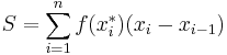
where xi-1 ≤ x*i ≤ xi. The choice of x*i in this interval is arbitrary. If x*i = xi-1 for all i, then S is called a left Riemann sum. If x*i = xi, then S is called a right Riemann sum. If x*i = (xi+xi-1)/2, then S is called a middle Riemann sum. The average of the left and right Riemann sum is the trapezoidal sum.
If it is given that
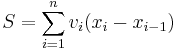
where vi is the supremum of f over [xi-1, xi], then S is defined to be an upper Riemann sum. Similarly, if vi is the infimum of f over [xi−1, xi], then S is a lower Riemann sum.
Any Riemann sum on a given partition (that is, for any choice of x*i between xi-1 and xi) is contained between the lower and the upper Riemann sums. A function is defined to be Riemann integrable if the lower and upper Riemann sums get ever closer as the partition gets finer and finer. This fact can also be used for numerical integration.
Methods
Riemann sum methods of x3 over [0,2] using 4 subdivisions
The four methods of Riemann summation are usually best approached with partitions of equal size. The interval ![[a,b]](/2012-wikipedia_en_all_nopic_01_2012/I/2c3d331bc98b44e71cb2aae9edadca7e.png) is therefore divided into
is therefore divided into  subintervals, each of length
  . The points in the partition will then be
 .
.
Left sum
For the left Riemann sum, approximating the function by its value at the left-end point gives multiple rectangles with base Δx and height f(a + iΔx). Doing this for i = 0, 1, ..., n−1, and adding up the resulting areas gives
![\Delta x \left[f(a) %2B f(a %2B \Delta x) %2B f(a %2B 2 \Delta x)%2B\cdots%2Bf(b - \Delta x)\right].\,](/2012-wikipedia_en_all_nopic_01_2012/I/26efdda527f37ebc3b54979b24dc00c6.png)
The left Riemann sum amounts to an overestimation if f is monotonically decreasing on this interval, and an underestimation if it is monotonically increasing.
Right sum
f is here approximated by the value at the right endpoint. This gives multiple rectangles with base Δx and height  . Doing this for
  , and adding up the resulting areas produces
![\Delta x \left[ f( a %2B \Delta x ) %2B f(a %2B 2 \Delta x)%2B\cdots%2Bf(b) \right].\,](/2012-wikipedia_en_all_nopic_01_2012/I/0472148aa6f45ea2e06a08a90a5e65c3.png)
The right Riemann sum amounts to an overestimation if  is monotonically increasing, and an underestimation if it is monotonically decreasing.
Middle sum
Approximating f at the midpoint of intervals gives f(a + Q/2) for the first interval, for the next one f(a + 3Q/2), and so on until f(b-Q/2). Summing up the areas gives
![Q\left[f(a %2B Q/2) %2B f(a %2B 3Q/2)%2B\cdots%2Bf(b-Q/2)\right].](/2012-wikipedia_en_all_nopic_01_2012/I/6577b8e73777fd7eb32405c08618596a.png)
The error of this formula will be
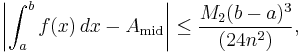
where  is the maximum value of the absolute value of
  on the interval.
Trapezoidal rule
In this case, the values of the function f on an interval are approximated by the average of the values at the left and right endpoints. In the same manner as above, a simple calculation using the area formula  for a trapezium with parallel sides b1, b2 and height h produces
![\frac{1}{2}Q\left[f(a) %2B 2f(a%2BQ) %2B 2f(a%2B2Q) %2B 2f(a%2B3Q)%2B\cdots%2Bf(b)\right].](/2012-wikipedia_en_all_nopic_01_2012/I/888c6bf9b41956b7a401223610b91ce1.png)
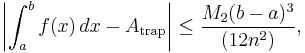
where is the maximum value of the absolute value of 
Examples
Example
Taking an example, the area under the curve of  between 0 and 2 can be procedurally computed using Riemann's method.
The interval from 0 to 2 is firstly divided into n subintervals, each of which is given a width of  ; these are the widths of the Riemann rectangles. Because the right Riemann sum is to be used, the sequence of x coordinates for the boxes will be
  . Therefore, the sequence of the heights of the boxes will be
  . It is an important fact that
  , and
, and  .
.
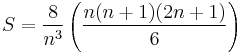
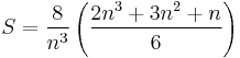
The area of each box will be  and therefore the nth right Riemann sum will be:
 . Hence:
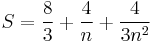
If the limit is viewed as  , it can be concluded that the approximation approaches the actual value of the area under the curve as the number of boxes increases. Hence:
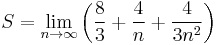

This method agrees with the definite integral as calculated in more mechanical ways:
Animations
See also
References
- Thomas, George B. Jr.; Finney, Ross L. (1996), Calculus and Analytic Geometry (9th ed.), Addison Wesley, ISBN 0-201-53174-7